MNIST是一个入门级的计算机视觉数据集。MNIST数据集的官网,我们可以手动下载数据集。
下载数据集
除了上面的手动下载数据集,tensorflow提供了一个库,可以直接用来自动下载MNIST。代码如下:
1 | from tensorflow.examples.tutorials.mnist import input_data |
运行上面的代码,会自动下载数据集并将文件解压到当前代码所在同级目录下的MNIST_data文件夹下。
注意:代码中的one_hot=True,表示将样本标签转化为one_hot编码。解释one_hot编码,假如一共10类。0的one_hot为1000000000,1的one_hot编码为0100000000,2的one_hot编码为0010000000,等等。只有一个位是1,1所在的位置就代表第几类,从零开始数。
MNIST数据集中的图片是28x28Pixel,所以,每一幅图就是1行784列的数据,每一个值代表一个像素。
如果是黑白的图片,图片中的黑色的地方数值为0,有图案的地方数值为0~255之间的数字,代表其颜色的深度。
如果是彩色的图片,一个像素由三个值表示RGB(红,黄,蓝)。
显示数据集信息
1 | print("输入数据为:",mnist.train.images) |
运行代码得出结果:

这是一个55000行、784列的矩阵,即:这个数据集有55000张图片。
MNIST数据集组成
在MNIST训练数据集中,mnist.train.images是一个形状为[55000,784]的张量。其中,第一个维度数字用来索引图片,第二个维度数字用来索引每张图片中的像素点。此张量里的每一个元素,都表示某张图片里的某个像素的强度值,值介于0~255之间。
MNIST数据集里包含三个数据集:训练集、测试集、验证集。训练集用于训练,测试集用于评估训练过程中的准确度,验证集用于评估最终模型的准确度。可使用以下命令查看里面的数据信息
1 | print("测试集的shape:",mnist.test.images.shape) |
运行完上面代码,可以发现在测试数据集里有10000条样本图片,验证集有5000个图片。
三个数据集还有分别对应的三个标签文件,用来标注每个图片上的数字是几。把图片和标签放在一起,称为“样本”。
MNIST数据集的标签是介于0~9之间的数字, 用来描述给定图片里表示的数字。标签数据是“one-hot vectors”: 一个one-hot向量,除了某一位的数字是1外, 其余各维度数字都是0。 例如, 标签0将表示为([1, 0, 0, 0, 0, 0,0, 0, 0, 0, 0]) 。 因此, mnist.train.labels是一个[55000, 10]的数字矩阵。
定义变量
1 | import tensorflow as tf |
代码中的None,代表此张量的第一个维度可以是任意长度的。
构建模型
定义学习参数
模型也需要权重值和偏置值,它们被统一称为学习参数。在Tensorflow,使用Variable来定义学习参数。
1 | W=tf.Variable(tf.random_normal([784,10])) |
定义正向传播
1 | pred=tf.nn.softmax(tf.matual(x,W)+b) |
定义反向传播
1 | #损失函数 |
首先,将正向传播生成的pred与样本标签y进行一次交叉熵的运算,然后取平均值。接着将cost作为一次正向传播的误差,通过梯度下降的优化方法找到能够使这个误差最小化的W和b。整个过程就是不断让损失值变小。因为损失值越小,才能表明输出的结果跟标签数据越接近。
训练模型
1 | #要把整个训练样本集迭代25次 |
测试模型
测试错误率的算法是:直接判断预测的结果与真实的标签是否相同,如是相同的就表示是正确的,如是不相同的,就表示是错误的。然后将正确的个数除以总个数,得到的值即为正确率。由于是one-hot编码,这里使用了tf.argmax函数返回one-hot编码中数值为1的哪个元素的下标。1代表横轴,0代表纵轴
1 | # 测试 model |
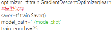
保存模型
在代码的两处区域加入以下代码:

读取模型
1 | print("开始第二个会话") |
完整代码
1 | import tensorflow as tf |
第70、71行的代码可以用68、69行的代码代替。pylab库结合了pyplot模块和numpy模块。