K-means

无监督学习与聚类算法

有监督学习的模型在训练的时候,即需要特征矩阵X,也需要真实标签y。机器学习当中,还有相当一部分算法属于“无监督学习”,无监督的算法在训练的时候只需要特征矩阵X,不需要标签。而聚类算法,就是无监督学习的代表算法。 聚类算法又叫做“无监督分类”,其目的是将数据划分成有意义或有用的组(或簇)。这种划分可以基于我们的业务需求或建模需求来完成,也可以单纯地帮助我们探索数据的自然结构和分布。

聚类算法在sklearn中有两种表现形式,一种是类(和我们目前为止学过的分类算法以及数据预处理方法们都一样),需要实例化,训练并使用接口和属性来调用结果。另一种是函数(function),只需要输入特征矩阵和超参数,即可返回聚类的结果和各种指标。

KMeans是如何工作的

关键概念:簇与质心

​ 簇:KMeans算法将一组N个样本的特征矩阵x划分为k个无交集的簇,直观上来看是簇是一组组聚集在一起的数据,在一个簇中的数据被认为是同一类。簇就是聚类的结果表现。

​ 质心:簇中所有数据的均值通常被称为这个簇的质心。在一个二维平面中,一簇数据点的质心的横坐标就是这一簇数据点的横坐标的均值,质心的纵坐标就是这一簇数据点纵坐标的均值。同理可推广到高维空间。

在KMeans算法中,簇的个数K是一个超参数,需要我们人为输入来确定。KMeans的核心任务就是根据我们设定好的K,找出K个最优的质心,并将离这些质心最近的数据分别分配到这些质心代表的簇中去。具体过程可以总结如下 :

​ 1、随机抽取k个样本作为最初的质心

​ 2、开始循环

​ 2.1、将每个样本点分配到离他们最近的质心,生成k个簇

​ 2.2、对于每个簇,计算所有被分到该簇的样本点的平均值作为新的质心

​ 3、当质心的位置不在发生变化,迭代停止,聚类完成

那什么情况下,质心的位置会不再变化呢?当我们找到一个质心,在每次迭代中被分配到这个质心上的样本都是一致的,即每次新生成的簇都是一致的,所有的样本点都不会再从一个簇转移到另一个簇,质心就不会变化了。

对于一个簇来说,所有样本点到质心的距离之和越小,我们就认为这个簇中的样本越相似,簇内差异就越小。而距
离的衡量方法有多种,令x表示簇中的一个样本点,ui表示该簇中的质心,n表示每个样本点中的特征数目,i表示组
成点x的每个特征,则该样本点到质心的距离可以由以下距离来度量:

如我们采用欧几里得距离,则一个簇中所有样本点到质心的距离的平方和为:

其中,m为一个簇中样本的个数,j是每个样本的编号。这个公式被称为簇内平方和(cluster Sum of Square),又叫做Inertia。而将一个数据集中的所有簇的簇内平方和相加,就得到了整体平方和(Total Cluster Sum ofSquare),又叫做total inertia。Total Inertia越小,代表着每个簇内样本越相似,聚类的效果就越好。因此,KMeans追求的是,求解能够让Inertia最小化的质心。实际上,在质心不断变化不断迭代的过程中,总体平方和是越来越小的。我们可以使用数学来证明,当整体平方和最小的时候,质心就不再发生变化了。如此,K-Means的求解过程,就变成了一个最优化问题

损失函数本质是用来衡量模型的拟合效果的,只有有着求解参数需求的算法,才会有损失函数。Kmeans不求解什么参数,它的模型本质也没有在拟合数据,而是在对数据进行一种探索。所以,K-Means不存在什么损失函数。Inertia更像是Kmeans的模型评估指标,而非损失函数。

重要参数和属性

参数

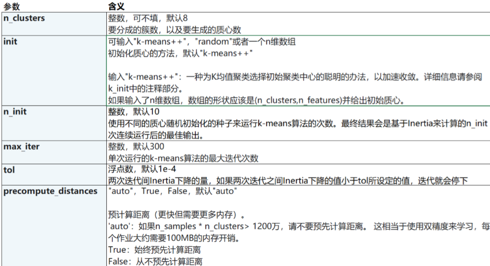
n_clusters是KMeans中的k,表示着我们告诉模型我们要分几类。这是KMeans当中唯一一个必填的参数,默认为8类,但通常我们的聚类结果会是一个小于8的结果。通常,在开始聚类之前,我们并不知道n_clusters究竟是多少,因此我们要对它进行探索。

在之前描述K-Means的基本流程时我们提到过,当质心不再移动,Kmeans算法就会停下来。但在完全收敛之前, 我们也可以使用max_iter,大迭代次数,或者tol,两次迭代间Inertia下降的量,这两个参数来让迭代提前停下 来。有时候,当我们的n_clusters选择不符合数据的自然分布,或者我们为了业务需求,必须要填入与数据的自然 分布不合的n_clusters,提前让迭代停下来反而能够提升模型的表现。

max_iter:整数,默认300,单次运行的k-means算法的大迭代次数
tol:浮点数,默认1e-4,两次迭代间Inertia下降的量,如果两次迭代之间Inertia下降的值小于tol所设定的值,迭代就会停下

属性

labels_:查看聚好的类别,每个样本所对应的类

cluster_centers_:查看质心

inertia_:查看总距离平方和

n_iter_:实际的迭代次数

coding:

1
2
3
4
5
6
7
8
9
10
11
12
13
14
15
16
17
18
19
20
21
22
23
24
25
26
27
28
29
30
31
32
33
34
35
36
37
38
39
40
41
42
43
44
45
46
47
48
49
50
51
52
53
54
55
56
57
58
59
60
61
62
63
64
65
66
67
68
from sklearn.datasets import make_blobs
import matplotlib.pyplot as plt
#这是自己制造数据集,n_samples代表数据个数,n_features代表数据特征个数
#random_state代表随机性
X, y = make_blobs(n_samples=500,n_features=2,centers=4,random_state=1)
fig, ax1 = plt.subplots(1)
ax1.scatter(X[:, 0], X[:, 1]#画点图
,marker='o'#代表点的形状
,s=8)#代表点的大小
#最开始数据集的形状
plt.show()
color = ["red","pink","orange","gray"]
fig, ax1 = plt.subplots(1)
for i in range(4):
ax1.scatter(X[y==i, 0], X[y==i, 1]
,marker='o'
,s=8
,c=color[i])
plt.show()
from sklearn.cluster import KMeans
#簇为3
n_clusters = 3
cluster = KMeans(n_clusters=n_clusters, random_state=0).fit(X)
#查看聚好的列表
y_pred = cluster.labels_
pre = cluster.fit_predict(X)
#查看质心
centroid = cluster.cluster_centers_
#查看总距离平方和
inertia = cluster.inertia_
print(inertia)
color = ["red","pink","orange","gray"]
fig, ax1 = plt.subplots(1)
for i in range(n_clusters):
ax1.scatter(X[y_pred==i, 0], X[y_pred==i, 1]
,marker='o'
,s=8
,c=color[i])
#画出质心
ax1.scatter(centroid[:,0],centroid[:,1]
,marker="x"
,s=15
,c="black")
plt.show()
#簇为4
n_clusters=4
cluster = KMeans(n_clusters=n_clusters, random_state=0).fit(X)
#查看聚好的列表
y_pred = cluster.labels_
pre = cluster.fit_predict(X)
#查看质心
centroid = cluster.cluster_centers_
#查看总距离平方和
inertia = cluster.inertia_
print(inertia)
color = ["red","pink","orange","gray"]
fig, ax1 = plt.subplots(1)
for i in range(n_clusters):
ax1.scatter(X[y_pred==i, 0], X[y_pred==i, 1]
,marker='o'
,s=8
,c=color[i])
#画出质心
ax1.scatter(centroid[:,0],centroid[:,1]
,marker="x"
,s=15
,c="black")
plt.show()

聚类算法的模型评估

上面的算法的簇随着数字的增大,总的距离和在不断的变小。难道我们我们就这样实验得出簇的个数吗?难道簇越小越好吗?看看算法的评估。聚类模型的结果不是某种标签输出,并且聚类的结果是不确定的,其优劣由业务需求或者算法需求来决定,并且没有永远的正确答案。那我们如何衡量聚类的效果呢? KMeans的目标是确保“簇内差异小,簇外差异大”,我们就可以通过衡量簇内差异来衡量聚类的效果。我们刚才说过,Inertia是用距离来衡量簇内差异的指标,因此,我们是否可以使用Inertia来作为聚类的衡量指标呢?Inertia越小模型越好嘛。可以,但是这个指标的缺点和极限太大。

当真实标签未知的时候使用轮廓系数

这样的聚类,是完全依赖于评价簇内的稠密程度(簇内差异小)和簇间的离散程度(簇外差异大)来评估聚类的效果。其中轮廓系数是最常用的聚类算法的评价指标。它是对每个样本来定义的,它能够同时衡量:
1)样本与其自身所在的簇中的其他样本的相似度a,等于样本与同一簇中所有其他点之间的平均距离
2)样本与其他簇中的样本的相似度b,等于样本与下一个最近的簇中得所有点之间的平均距离根据聚类的要求”簇内差异小,簇外差异大“,我们希望b永远大于a,并且大得越多越好。单个样本的轮廓系数计算为

这个公式可以看作:

很容易理解轮廓系数范围是(-1,1),其中值越接近1表示样本与自己所在的簇中的样本很相似,并且与其他簇中的样本不相似,当样本点与簇外的样本更相似的时候,轮廓系数就为负。当轮廓系数为0时,则代表两个簇中的样本相似度一致,两个簇本应该是一个簇。

在sklearn中,我们使用模块metrics中的类silhouette_score来计算轮廓系数,它返回的是一个数据集中,所有样本的轮廓系数的均值。但我们还有同在metrics模块中的silhouette_sample,它的参数与轮廓系数一致,但返回的是数据集中每个样本自己的轮廓系数。

1
2
3
4
5
#接上面的代码
from sklearn.metrics import silhouette_samples
from sklearn.metrics import silhouette_score
print("4个簇的时候的轮廓系数:",silhouette_score(X,y_pred))
print("四个簇的每个样本的轮廓系数:",silhouette_samples(X,y_pred))

当真实标签未知的时候用CHI

除了轮廓系数是常用的,我们还有卡林斯基-哈拉巴斯指数(Calinski-Harabaz Index,简称CHI,也被称为方差比标准),戴维斯-布尔丁指数(Davies-Bouldin)以及权变矩阵(Contingency Matrix)可以使用。

在这里我们重点来了解一下卡林斯基-哈拉巴斯指数。Calinski-Harabaz指数越高越好。对于有k个簇的聚类而言,Calinski-Harabaz指数s(k)写作如下公式:

其中N为数据集中的样本量,k为簇的个数(即类别的个数),Bk是组间离散矩阵,即不同簇之间的协方差矩阵, Wk是簇内离散矩阵,即一个簇内数据的协方差矩阵,而tr表示矩阵的迹。在线性代数中,一个n×n矩阵A的主对角线(从左上方至右下方的对角线)上各个元素的总和被称为矩阵A的迹(或迹数),一般记作tr(A) 。数据之间的离散程度越高,协方差矩阵的迹就会越大。组内离散程度低,协方差的迹就会越小,Tr(Wk)也就越小,同时,组间离散程度大,协方差的的迹也会越大, Tr(Bk)就越大,这正是我们希望的,因此Calinski-harabaz指数越高越好。

1
2
3
#接上面的代码
from sklearn.metrics import calinski_harabaz_score
print(calinski_harabaz_score(X, y_pred))

基于轮廓系数选择簇的个数

1
2
3
4
5
6
7
8
9
10
11
12
13
14
15
16
17
18
19
20
21
22
23
24
25
26
27
28
29
30
31
32
33
34
35
36
37
38
39
40
41
42
43
44
45
46
47
48
49
50
51
52
53
54
55
56
57
58
59
60
61
62
63
64
65
66
67
68
69
70
71
72
73
74
75
76
77
78
79
80
81
82
83
84
85
86
87
88
89
90
91
92
93
94
95
96
97
98
99
100
101
102
103
104
105
106
107
from sklearn.datasets import make_blobs
import matplotlib.pyplot as plt
from sklearn.metrics import silhouette_samples
from sklearn.metrics import silhouette_score
from sklearn.cluster import KMeans
import matplotlib.cm as cm
import numpy as np
#自己制造数据集,n_samples代表数据个数,n_features代表数据特征个数
#random_state代表随机性
X, y = make_blobs(n_samples=500,n_features=2,centers=4,random_state=1)
n_clusters = 4
fig, (ax1, ax2) = plt.subplots(1, 2)
fig.set_size_inches(18, 7)
ax1.set_xlim([-0.1, 1])
ax1.set_ylim([0, X.shape[0] + (n_clusters + 1) * 10])
clusterer = KMeans(n_clusters=n_clusters, random_state=10).fit(X)
cluster_labels = clusterer.labels_
silhouette_avg = silhouette_score(X, cluster_labels)
print("For n_clusters =", n_clusters,
"The average silhouette_score is :", silhouette_avg)
sample_silhouette_values = silhouette_samples(X, cluster_labels)
y_lower = 10
for i in range(n_clusters):
ith_cluster_silhouette_values = sample_silhouette_values[cluster_labels == i]
ith_cluster_silhouette_values.sort()
size_cluster_i = ith_cluster_silhouette_values.shape[0]
y_upper = y_lower + size_cluster_i
color = cm.nipy_spectral(float(i)/n_clusters)
ax1.fill_betweenx(np.arange(y_lower, y_upper)
,ith_cluster_silhouette_values
,facecolor=color
,alpha=0.7)
ax1.text(-0.05
, y_lower + 0.5 * size_cluster_i
, str(i))
y_lower = y_upper + 10
ax1.set_title("The silhouette plot for the various clusters.")
ax1.set_xlabel("The silhouette coefficient values")
ax1.set_ylabel("Cluster label")
ax1.axvline(x=silhouette_avg, color="red", linestyle="--")
ax1.set_yticks([])
ax1.set_xticks([-0.1, 0, 0.2, 0.4, 0.6, 0.8, 1])
colors = cm.nipy_spectral(cluster_labels.astype(float) / n_clusters)
ax2.scatter(X[:, 0], X[:, 1]
,marker='o' #点的形状
,s=8 #点的大小
,c=colors)
centers = clusterer.cluster_centers_
ax2.scatter(centers[:, 0], centers[:, 1], marker='x',
c="red", alpha=1, s=200)
ax2.set_title("The visualization of the clustered data.")
ax2.set_xlabel("Feature space for the 1st feature")
ax2.set_ylabel("Feature space for the 2nd feature")
plt.suptitle(("Silhouette analysis for KMeans clustering on sample data "
"with n_clusters = %d" % n_clusters),
fontsize=14, fontweight='bold')
plt.show()
for n_clusters in [2,3,4,5,6,7]:
n_clusters = n_clusters
fig, (ax1, ax2) = plt.subplots(1, 2)
fig.set_size_inches(18, 7)
ax1.set_xlim([-0.1, 1])
ax1.set_ylim([0, X.shape[0] + (n_clusters + 1) * 10])
clusterer = KMeans(n_clusters=n_clusters, random_state=10).fit(X)
cluster_labels = clusterer.labels_
silhouette_avg = silhouette_score(X, cluster_labels)
print("For n_clusters =", n_clusters,
"The average silhouette_score is :", silhouette_avg)
sample_silhouette_values = silhouette_samples(X, cluster_labels)
y_lower = 10
for i in range(n_clusters):
ith_cluster_silhouette_values = sample_silhouette_values[cluster_labels == i]
ith_cluster_silhouette_values.sort()
size_cluster_i = ith_cluster_silhouette_values.shape[0]
y_upper = y_lower + size_cluster_i
color = cm.nipy_spectral(float(i)/n_clusters)
ax1.fill_betweenx(np.arange(y_lower, y_upper)
,ith_cluster_silhouette_values
,facecolor=color
,alpha=0.7
)
ax1.text(-0.05
, y_lower + 0.5 * size_cluster_i
, str(i))
y_lower = y_upper + 10
ax1.set_title("The silhouette plot for the various clusters.")
ax1.set_xlabel("The silhouette coefficient values")
ax1.set_ylabel("Cluster label")
ax1.axvline(x=silhouette_avg, color="red", linestyle="--")
ax1.set_yticks([])
ax1.set_xticks([-0.1, 0, 0.2, 0.4, 0.6, 0.8, 1])
colors = cm.nipy_spectral(cluster_labels.astype(float) / n_clusters)
ax2.scatter(X[:, 0], X[:, 1]
,marker='o' #点的形状
,s=8 #点的大小
,c=colors
)
centers = clusterer.cluster_centers_
ax2.scatter(centers[:, 0], centers[:, 1], marker='x',
c="red", alpha=1, s=200)
ax2.set_title("The visualization of the clustered data.")
ax2.set_xlabel("Feature space for the 1st feature")
ax2.set_ylabel("Feature space for the 2nd feature")
plt.suptitle(("Silhouette analysis for KMeans clustering on sample data "
"with n_clusters = %d" % n_clusters),
fontsize=14, fontweight='bold')
plt.show()
----本文结束,感谢您的阅读。如有错,请指正。----
大哥大嫂过年好!支持我一下呗
0%